Here is the final demo video:

SSAO Blur

To calculate SSAO, I randomly rotated the kernel for each fragment, I was able to get high-quality results with a small number of samples. This did come at a price as the randomness introduced a noticeable noise pattern. John Chapman says that we can fix the problem by blurring the results.

Here is an image of the visible noise pattern.
(For better visualization, please open the image in a new tab/window )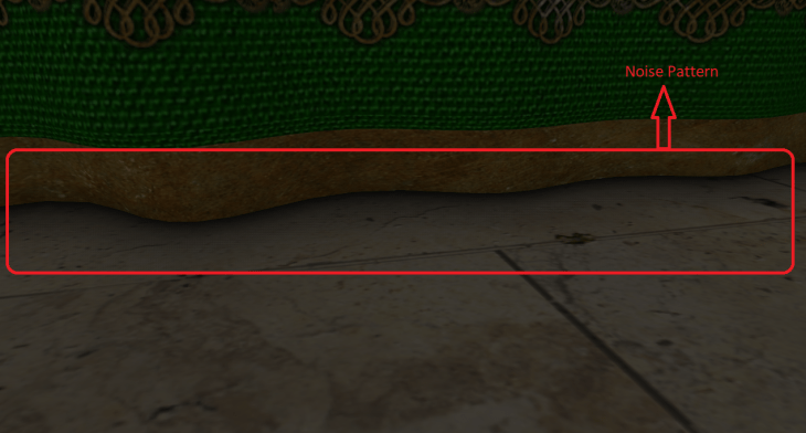

So I added another pass to blur the result of SSAO. The result of the SSAO blur pass is again an ambient occlusion factor but this time it is without the noise pattern problems. To store the blurred ambient occlusion factor, I created another frame buffer and bound it in the SSAO blur pass. The vertex shader for the SSAO blur did 1 job i.e. to pass the texture coordinates to the fragment shader. So I used the same vertex shader that the SSAO pass was using. The fragment shader of the SSAO blur pass calculated the surrounding texels around the fragment, sampled the ambient occlusion (using SSAO texture) for the surrounding texels, computed the average for the sampled ambient occlusion and assigned it to the SSAO blur texture. This calculation was done for all the fragments. But how were the surrounding texels calculated? As I already knew the size of my noise texture (4×4 in my case), I used this to my advantage. I traversed between -noiseTexturedDimension/2 to +noiseTexturedDimension/2 both horizontally and vertically to get the surrounding texels (from -2.0 to 2.0 in my case).

Here is how the output looked after applying the blur results.

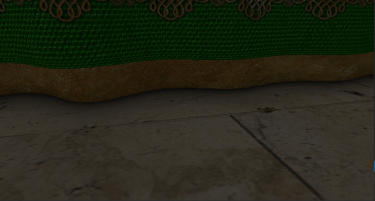
As you can see, the noise pattern is smoothly removed.

ImgUI

There were some number of variables that I could tweak to get variable results from the SSAO pass.

• SSAO Kernel Size (number of samples)
• SSAO Radius
• SSAO Bias
• SSAO Power

Along with these variables, I wanted to enable/disable SSAO pass and SSAO blur pass to visualize the the output with & without SSAO. I could have easily implemented this by creating boolean & float variables and varied them with the key bindings using glfw. This would have worked, but it wouldn’t have been visually interesting. So I wanted some sort of visual representation for these variables which I could vary, like a UI. Creating a UI by myself would have taken a lot of time and that wasn’t the point of the project, so I started searching for some existing libraries. In that process, I came across the library called ImgUI. This library was small, free to use and was easy to implement. So I included the library into my project and threw all my tweakable variables into the UI. I added checkboxes to enable/disable SSAO pass and SSAO blur pass, I added sliders to vary SSAO Kernel Size, SSAO Radius, SSAO Bias and SSAO Power.

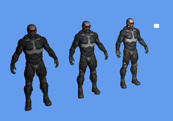
Here’s how the output looked after implementing ImgUI (A.K.A dear imgUI):

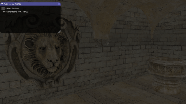
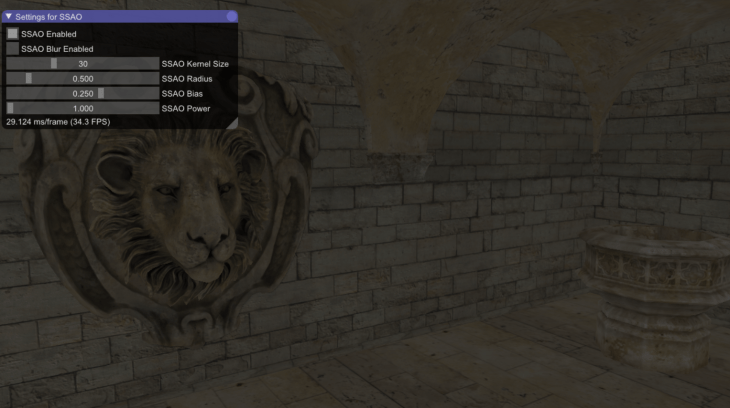
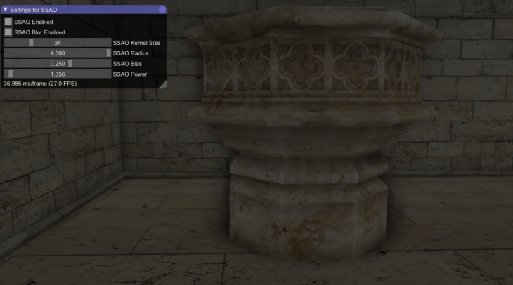
The SSAO radius is increased in the third image. Because of that, as you can see, the ambient occlusion on the pillar spreads outwards.

After reading about SSAO. For the week 7, I took the first shot at implementing it.

I currently have 3 passes in my implementation before the final output shows on screen.

1. Geometry pass
2. SSAO pass
3. Lighting pass

Geometry pass: The functionality of the geometry pass remains the same; like the one, I had for deferred rendering.

• I create a frame buffer (G-buffer).
• I create 3 color buffers and bind it to the G-buffer.
  • Color buffer 0: To store all the vertex positions (RGB).
  • Color buffer 1: To store all the normals (RGB).
  • Color buffer 2: To store diffuse and specular textures (RGBA).
• I create a depth buffer (render buffer) and bind it to the G-buffer.

I bind the G-buffer in the geometry pass, pass in the model, view, & projection matrices as uniforms to the shaders. The fragment shader for the geometry pass is the same as I had before: I store the positions(Color buffer 0) and normals(Color buffer 1) in the framebuffers, I sample the diffuse and specular textures(Color buffer 2) and again store them in the framebuffers. There is one small change in the vertex shader though, i.e. instead of transforming the positions and normals to the world space, I transform them to the view space and then pass them to the fragment shader.

After storing all the necessary geometric information in the G-buffer, it was time to compute the ambient occlusion factor (in SSAO pass).

SSAO pass: To calculate the ambient occlusion factor, I needed positions, normals and a random vector for each fragment. I need the random vector to calculate the orthonormal basis for TBN matrix (Orthonormal basis TBN matrix is used to orient the samples along the surface of the fragments). As it is expensive to calculate a random vector for each fragment, I stored a 4×4 texture of random vectors, wrapped it to repeat mode and sampled them in the SSAO fragment shader. So I bound a total of 3 textures in the SSAO pass.

1. Positions
2. Normals
3. 4×4 texture of random vectors

The result of the SSAO pass would be an ambient occlusion factor which will be used in the lighting pass. So after performing SSAO calculations, I had to pass in the occlusion factor to the lighting pass. For this reason, I created another framebuffer and bound it in the SSAO pass.

The vertex shader of the SSAO pass did a single job i.e. to pass the texture coordinates to the fragment shader.

The fragment shader is where all the major calculations happened. I first created a tangent vector which was orthogonal to the normal vector. I used Gramm-Schmidt’s process (project the sampled random vector onto the normal and then subtract the projected vector with the random vector which gives a direction vector orthogonal to the normal) to obtain the tangent vector. I then applied cross-product to the normal and the tangent vector to get another vector (bitangent) which was orthogonal to both the normal and the tangent vector. With all the 3 orthogonal vectors in hand, I created a TBN matrix.

After creating the TBN matrix, I looped through all the samples of the kernel and:

• Oriented the samples to the surface of the fragment by multiplying the samples with the TBN matrix.
• Transformed the samples from the tangent space to the view space by adding the samples (sample values would previously be: -1 =< X =< 1, -1 =< Y =< 1, 0 =< Z =< 1 ) with the fragment position. Before doing this, I also multiplied the samples with a radius value. This radius value can be visualized as the radius of the hemisphere, in future, this value can be varied to get different effects from the SSAO calculation. After transforming the samples to view space, we can visualize the samples as though they are surrounding the fragment in all directions.
• Multiplied the samples with the projection matrix to get the samples in projection space. I also performed perspective division for the samples (Generally, this operation is automatically performed at the end of the vertex shader).
• I then sampled these samples (which are now present in screen space) with the position texture to retrieve the Z (sampled depth) value.
• Now I check if the sampled depth value is within the radius that we specified (range check). This range check is important, especially for the fragments that make up the edges of the meshes.
• If the sampled depth is within the radius and is greater than the depth of the fragment then I increment 1 to the occlusion factor.

After looping through all the samples I get the number of samples whose depth value is greater than the depth value of the fragment. Let’s call it ‘occlusionNumber’. I then divide the ‘occlusionNumber’ with the total number of samples and subtract it with 1.0 to get the exact ambient occlusion factor. I store this ambient occlusion factor in the SSAO frame buffer.

3. Lighting pass: Previously I only used positions, normals, diffuse and specular textures for the lighting pass (i.e. to calculate lighting). This time, I also have the ambient occlusion factor to help me with the lighting calculation. So along with the other framebuffers, I also bound the SSAO framebuffer as a uniform (which contained the occlusion factor) to the shader. I added a simple point light to my demo and performed lighting calculations. The occlusion factor was multiplied in a straightforward fashion to the ambient light component which contributed to the final color of the fragment.

Here is a side-by-side comparison of how the output looked without and with SSAO.

Without SSAO:

With SSAO:

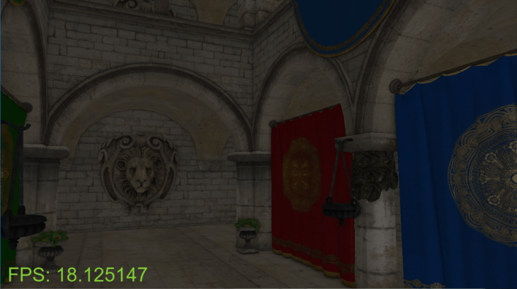
Here is a .gif image for better visualization:

As you can see, the framerate has drastically dropped from 67-90 fps to 17-20 fps with the screen size 1280 x 720. I was able to pump the framerate to 35-38 fps by reducing the samples from 64 to 32.

After rendering the scene with deferred rendering pipeline, I started with Screen Space Ambient Occlusion for the 6th week of my project.

In reality, when the light is projected on an object, it scatters in all directions with varying intensities, so the indirectly lit parts of a scene should also have varying intensities. One type of indirect lighting approximation is called ambient occlusion that tries to approximate indirect lighting by darkening creases, holes and surfaces that are close to each other. These areas are largely occluded by surrounding geometry and thus light rays have fewer places to escape, hence the areas appear darker.

Ambient occlusion techniques are expensive as they have to take surrounding geometry into account. In 2007 Crytek published a technique called screen-space ambient occlusion (SSAO) for use in their title Crysis. This technique uses the scene’s depth in screen-space to determine the amount of occlusion instead of real geometrical data. This approach is incredibly fast compared to real ambient occlusion and gives plausible results.

I’m referring to John Chapman’s SSAO tutorial for my implementation.

The idea behind screen-space ambient occlusion is simple: for each fragment on a screen-filled quad we calculate an occlusion factor based on the fragment’s surrounding depth values. The occlusion factor is then used to reduce or nullify the fragment’s ambient lighting component. The occlusion factor is obtained by taking multiple depth samples in a sphere sample kernel surrounding the fragment position and compare each of the samples with the current fragment’s depth value. The number of samples that have a higher depth value than the fragment’s depth represents the occlusion factor.

It is clear that the quality of this technique is directly related to the number of surrounding samples we take. If the sample count is too low the quality/precision reduces drastically and we get an artifact called banding; if it is too high we lose performance. John Chapman says that we can reduce the number of samples we have to test by introducing some randomness into the sample kernel. By randomly rotating the sample kernel each fragment we can get high-quality results with a much smaller amount of samples. But the randomness also introduces a noticeable noise pattern. He says that we can fix it by blurring the results.

In Crysis, as the kernel used was a sphere, it caused flat walls to look gray as half of the kernel samples end up being in the surrounding geometry. For this reason, John Chapman suggests using a hemisphere instead of a sphere which can be oriented along the surface’s normal vector. By sampling around this normal-oriented hemisphere we do not consider the fragment’s underlying geometry as a contribution to the occlusion factor. This removes the gray-feel of ambient occlusion.

So for this week, I studied in detail about how to implement SSAO. I also had to learn about Gramm-Schmidt process which helps me in creating an orthogonal basis.

So why do we need an orthogonal basis? As it is difficult nor plausible to generate a sample kernel for each surface normal direction we can generate a sample kernel in tangent-space, with the normal vector pointing in the positive z direction. To then transform the samples from tangent-space to view-space, I need a TBN (tangent, bi-tangent, & normal) matrix. To create the TBN matrix, I need a normal, tangent and bi-tangent vector. All of these vectors are orthogonal to each other. I already have the normal vector that I get while loading a model. To calculate the tangent, I use a random vector and use the Gramm-Schmidt process to get the vector orthogonal to the normal. I can then cross-product with the normal and the tangent vector to get the bi-tangent vector. Using these 3 orthogonal vectors, I can then create a TBN matrix.

Content under development.

After rendering lights with forward rendering, I wanted to start implementing deferred rendering. So for week 4, I took a shot at the first pass of deferred rendering.

Before going into deferred rendering, let me point out the disadvantages of forward rendering:

1. Each rendered object has to iterate over each light source for every rendered fragment which is a lot!
2. Forward rendering also tends to waste a lot of fragment shader runs when multiple objects cover the same screen pixels as most fragment shader outputs are overwritten (lighting calculations were wasted on them).

Deferred rendering/shading tries to overcome the issues of forward rendering which drastically changes the way objects are rendered. It provides several options to significantly optimize scenes which allows us to render hundreds or even thousands of lights with an acceptable framerate. Deferred shading is based on the idea that we defer or postpone most of the heavy rendering, like lighting to a later stage. It consists of two passes, the Geometry pass and the Lighting pass.

1. Geometry pass: We render the scene once and retrieve all kinds of geometrical information from the objects that we store in a collection of textures called the G-buffer. Geometrical information includes position vectors, color vectors, normal vectors and/or specular values. So I wrote a vertex and a fragment shader to do exactly the same. My vertex shader looked almost the same as before, but my fragment shader completely changed. Instead of calculating lighting and outputting the color to the fragments, the fragment shader stored positions, normals, albedo(diffuse color) and specular values to the framebuffer(G-buffer) like a texture data. (G-buffer is the collective term for all textures used to store lighting-relevant data for the final lighting pass)

To store the geometrical information into the G-buffer from the pixel shader, I first had to create a framebuffer, generate and bind the textures to the framebuffer with a color attachment number. I used the same attachment number as the layout location specifier in the fragment shader, something like:
layout (location = 0) out vec3 gPosition;
layout (location = 1) out vec3 gNormal;
The dimensions of all the frame buffers, were exactly the same as the dimensions of the window.

2. Lighting pass: We render a screen-filled quad and calculate the scene’s lighting for each fragment using the geometrical information stored in the G-buffer. We iterate pixel by pixel over the G-buffer. I wrote another vertex shader and fragment shader for the lighting pass. The vertex shader was simple, it just took the positions and texture coordinates as it’s input. The positions and texture co-ordinates were the entire screen coordinates in normalized device coordinates. The vertex shader just set the position of each vertex using gl_position as before and passed the texture coordinates to the fragment shader. The fragment shader in lighting pass is where all the heavy calculations were performed. (I implemented ambient and specular lighting for this week). The main difference between the fragment shader in the forward rendering and deferred rendering was that, in forward rendering, I was sampling diffuse and specular textures from the uniforms currently bound to it. However, in deferred rendering, the textures were sampled from the framebuffer(G-buffer) that were stored in the geometry pass. Along with the textures, I also fetched the fragment’s position vectors and normal vectors from the framebuffer rather than from being passed from the vertex shader like forward rendering.

Here is how the output looked after implementing deferred rendering.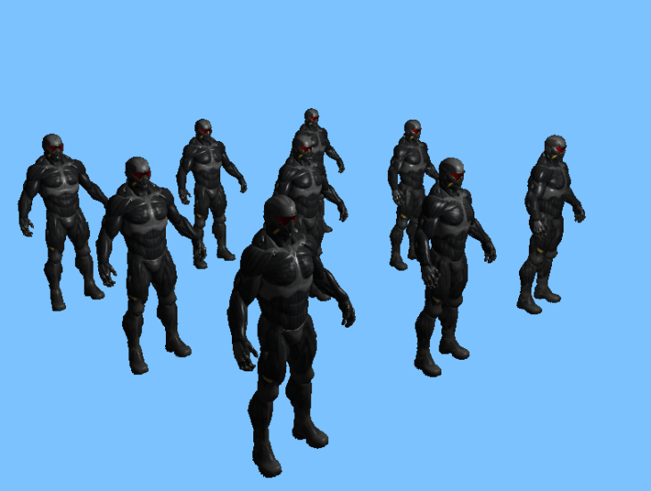

The output looks similar to forward rendering. The point is that if we implement n-number of lights with deferred rendering, there wouldn’t be a significant drop in the frame rate which would have not been possible with forward rendering.

I wanted to implement lights for the third week of my project. I wanted to implement directional, ambient, specular, point and spot lights.

Directional Light: Directional light is simple to visualize and understand. The closer the fragments of an object are aligned to the light rays, the more the brightness are of those fragments.

It is amazing how the dot product of two directional vectors work. The dot product of two directional vectors results in 0.0 when they are perpendicular and 1.0 when they are parallel. So the dot product increases from 0.0 to 1.0 as the vectors get closer in direction. So to light the fragments, I knew I needed the light direction, normal of the surface, and the light color to light the fragments. I passed the light direction & the light color as parameters to the fragment shader, passed the normal(interpolated) of a vertex from vertex shader to the fragment shader. I then normalized the vectors, calculated the dot product between the normals and the light direction which resulted in the lighting factor. I applied the lighting factor along with the light color to the fragment shader’s output i.e the final color of the pixel.

Passing in the light source’s position instead of its direction and calculating the direction between the light and each fragment provided with more accurate lighting results.

Ambient Light: After applying directional light, the pixels that were facing opposite to the direction of the light source, were completely dark. So I wanted to implement ambient lighting. Realistically there is always some sort of light somewhere in the world even when it’s dark, so objects are almost never completely dark; example: Moon.

Ambient lighting is the simplest form of lighting. We just take an ambient factor (minimum amount of lighting to be applied to an object) from 0.0 to 1.0, multiply it with a light color and apply it to the final resulting pixel. Similar to the directional light, I passed in the ambient factor and ambient light color as parameters to the fragment shader, multiplied them and applied to the color of the pixel i.e. the fragment shader’s output. The light color of ambient light can also act as a tint to an object.

Specular Light: It simulates the bright spot of a light that appears on shiny objects. Specular highlights are often more inclined to the color of the light than the color of the object. Alike directional lighting, specular lighting is based on the light’s direction vector and the object’s normal vectors, but it is also based on the view direction or the camera’s direction, example: from what direction the player is looking at the fragment. To calculate the view direction, I had to pass in the view position to the fragment shader. I calculated the view direction from the view position and the fragment’s position (fragment position was passed in from the vertex shader). I then calculated the light’s reflection direction using GLSL’s reflect() which needed the light direction and the surface normal as its parameters. After getting the view direction and the light’s reflection direction, I calculated the dot product of the vectors and raised it to the power of the shininess factor (32 for example, higher the shininess factor, the smaller the highlight becomes) to get the specular factor. Similar to the other lights, I applied the specular factor along with the light color to the fragment shader’s output.

I could have also used blinn-phong’s model instead of phong’s model and calculated the specular lighting using the half vector. The shininess factor affects the lighting a bit differently in blinn-phong’s model.

Here is how the ouput looked after implementing directional, ambient and specular lighting. I have a white cube to indicate the position of the light source.

Point Light: It is a light source with a given position in the world that illuminates in all directions and the light rays fade out over a distance, example: light bulbs. For point lights, the light is generally quite bright when standing close by, but the brightness diminishes quickly at the start and the remaining light intensity diminishes slowly over distance. As the light rays travel over distance, it loses its intensity, this is generally called Attenuation. To calculate this attenuation factor I used the formula:

Fatt = 1.0 / (Kc + Kl ∗ d + Kq ∗ d2)

Where:

d: Is the distance from the fragment to the light source.

Kc: Is a constant term which I kept it at 1.0. This is usually kept at 1.0 to make sure the resulting denominator never gets smaller than 1.0.

Kl: A linear term that reduces the intensity of the light in a linear fashion.

Kq: A quadratic term which will be less significant compared to the linear term when the distance is small, but gets much larger than the linear term as the distance grows.

I had to pass in the constants Kc, Kl & Kq to the fragment shader to calculate the attenuation factor. After calculating the attenuation factor using the above-mentioned formula, I simply multiplied it with the directional light factor and specular light factor that I had previously calculated. This gave me a decent visualization of point light with its intensity decreasing over distance.

Here is how the output looked after implementing a point light. The cube indicates the position of the point light.

Spot Light: A spotlight is a light source that is located somewhere in the environment that, instead of shooting light rays in all directions (like point light), it only shoots them in a specific direction. The result is that only the objects within a certain radius of the spotlight’s direction are lit and everything else stays dark. A good example of a spotlight would be a street lamp or a flashlight.

To calculate the spotlight intensity, I had to first have a position for spotlight, specify its direction, inner radius, outer radius and pass them to the fragment shader. I start with, I had to calculate the spotlight direction relative to the fragment position,  I got it by subtracting the fragment’s position and spotlight’s position. After getting the relative direction, I applied the dot product between the spotlight direction and the relative direction which gave me a cosine of the angle between them i.e. from -1 to +1. The spotlight intensity is calculated only if the resultant value is > 0.0 i.e if the fragments are facing the direction of the spotlight. I used the GLSL’s smoothstep() function to perform Hermite interpolation between the spotlight’s inner radius and outer radius using the theta as the factor, which gave me the spotlight intensity. I then multiplied the spotlight intensity with the diffuse factor and the specular factor that I had calculated before.

Here is how the output looked after implementing a spotlight.

For the second week of the project, I wanted to render some cubes on the screen, set up a camera, load a model and texture the loaded model.

Rendering cubes: Before rendering anything that is 3D, I knew I had to set up a model, view and projection matrix.

I’m using glm’s mat4 (identity matrix) to perform the matrix operations.

• Model/World matrix: Used to transform the coordinates from object space to the world space. Translation, rotation & scaling is applied with the help of this matrix. I used glm’s translation(), rotation() & scaling() functions to transform the vertices from object space to world space.
• Projection matrix: Used to create a frustum that defines the visible space. Anything outside the frustum will not end up in the clip space volume and will thus become clipped. As I will be rendering cubes(3D), I need to have a 3D projection. I’m taking help of glm’s perspective() function to provide me a projection matrix. I had to set the field of view(45.0f), aspect ratio(width/height of screen), near plane(0.1f) and far plane(100.0f) for the function to give me a frustum projection matrix.
• View matrix: This is the matrix where the camera’s position and direction are set. But for rendering cubes, I just hard-coded the view position to a vector from where I could see the cubes.

I also enabled the depth testing using openGL’s glEnable(GL_ENABLE_TEST), so that a fragment that is behind another fragment is discarded which otherwise would have overwritten.

Here is how the output looked after rendering cubes.

Setting up camera: I wanted to set up an FPS-style camera with mouse movements similar to it. Camera moving forward and backward directions using W and S keys, left and right directions using A and D keys, additionally up and down directions using E and Q keys and zooming in and out using mouse’s scroll movement. All of these had to be applied to the view matrix. I used glm’s lookAt() to give me the view matrix. It took camera’s position, camera’s direction and camera’s up vector as its input. I took help of glfw and registered call backs to keyboard and mouse events.

The camera’s position was updated each time the user pressed any of the WASDQE keys with a constant camera speed. The normalized camera’s direction was updated each time the user moved the mouse. The camera’s zoom was updated each time (field of view from 1.0f to 45.0f) the user scrolled. As the camera’s direction changed for every mouse movement, I needed to calculate the camera’s up vector which was given to the lookAt(). I used the cross product of camera’s direction(Front) and Right vector to calculate the camera’s up vector.

Here is how the output looked after setting up the camera.

Loading and texturing a model: I’m the using assimp library to load models. I wanted the debug and release versions of the library for both x86 and x64 platforms. But the precompiled libraries that I downloaded from the assimp’s website didn’t contain all of them. Nuget packages were available for assimp but it provided me with an older version(3.0, released July 2012). So I decided to download the source code and compile it by myself.

CMake to the rescue. After downloading the source code I generated the visual studio solution files using CMake. I could then compile and generate the library files(.lib & .dll) for both the debug and release versions for the x86 platform. I wasn’t able to change the platform to x64 using visual studio’s configuration manager and generate the library files immediately. I searched and changed all the known places in the project properties and configuration manager to help change to x64 platform and get the library files. But the visual studio was only exporting the .lib file upon building and not the .dll file. It turns out that I had to generate the visual studio solution files(using CMake) for x64 and x86 separately. After knowing that, I changed the configuration settings in CMake and generated the solution files for x64 separately and successfully built the library files.

Anyways after building & linking the assimp library, I wrote a simple Mesh and Model class to store the vertices, indices, textures etc. I was able to load the model file using assimp’s ReadFile() function. (Assimp prefixes member variables with ‘m’ and their function names are in Pascal Case, which is how all of my code is. I learnt this style from my professor Paul Varcholik) After loading the model, I loaded all the vertices, indices and texture coordinates into my data structure. Assimp was also nice enough to give me the name of the textures associated with the loaded model. I then loaded the textures using stb_image like before and sampled them to the pixels.

Here is how the output looked after loading and applying texture to a model.

For the first week, I focused on setting up the project, rendering a triangle with a color applied on it and then rendering a square with textures applied on it.

Project Setup:  I’m using the following external libraries for the project.

• Glfw: For window creation, user input etc.
• Glad: To determine OpenGL extensions on the target platform.
• stb_image: To load textures of different format.
• Glm: To represent the math structures like vectors & matrices and perform math calculations like translation, rotating, scaling etc.

I created a window using Glfw, setup my viewport and created an update loop.

Rendering a triangle: Apparently, it takes some time to a render a triangle for the first time. I declared an array of floats for the vertices(NDC) of my triangle and placed them inside the vertex buffer. I specified the format of the vertex buffer which will be used by the shader. I wrote a simple vertex shader which sets the position of the vertices of the triangle. I also wrote a simple fragment shader which sets the color for each fragment to be rendered on the screen. The triangle was rendered with the color set in the fragment shader.

Rendering a square with textures: After rendering a triangle, I immediately moved on to render a square by using 2 triangles. I used the element buffer to avoid duplication of the vertices. I created an index array containing the order of the vertices to be drawn that make a square and placed them in the element buffer. I specified the format of the element buffer similar to how I specified the format of the vertex buffer. To apply the texture for the created square, I had to load the texture (using stb_image), bind it, set magnification and minification filtering properties for it and finally map its coordinates to the square. I added the texture coordinates into the previously specified vertex array which would be placed in the vertex buffer. I used the vertex shader to simply forward the texture coordinates to the fragment shader. I mapped the texture coordinates in the fragment shader. I also loaded another texture and mapped it on top of the square and added a simple rotation. Here is how the output looked after my first week of progress:

This is the first blog of my 9 week personal project: Screen Space Ambient Occlusion algorithm with Deferred Shading in C++ & OpenGL 4+. I will be writing blogs every week on my development progress of the project.